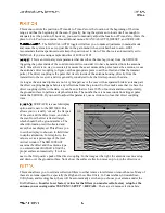
The input number here is scans, so in order to use this filter, find the length in scans of the feature that
you want to remove and put that number into the system. Features of this size or larger will be removed
from the data.
AGC stands for Automatic Gain Control. AGC lets you choose a set number of gain points (2, 3, or
5) distributed evenly through the vertical scale. The object of AGC is to normalize (make even-looking)
the scan by reducing the gain for areas where the signal is very strong (usually near the surface), but
adding gain with increasing attenuation (usually with depth). This dramatically slows the scroll speed of
the data, especially if 5 points are used. A faster option is Display Gain, located under the Display sub-
menu in Output.
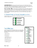
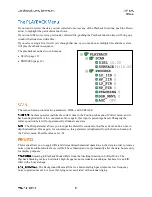
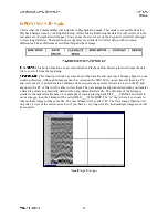
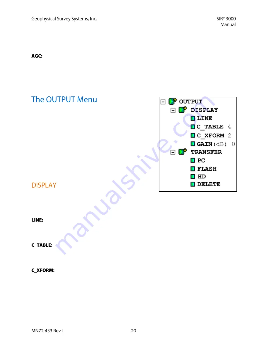
This menu controls the data display, printing, and file
maintenance. There are two sub-menus to the Output menu:
DISPLAY (page 20)
TRANSFER (page 21)
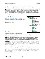
This sub-menu controls the ‘look and feel’ of the data
displayed on the screen. Here is where you can change the mode of display, color table and distribution
(transform), and add screen gain. There are four parameter inputs here: Mode (LINE/SCOPE),
C_TABLE, C_XFORM, and GAIN(dB).
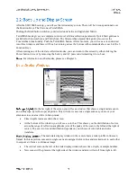
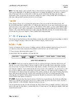
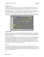
This is really the Mode option which allows you to toggle between Linescan and Scope display
modes. Linescan is the conventional way of looking at GPR data with each scan stacked next to its
neighbor and amplitude values along that scan assigned a color value. Scope, or oscilloscope, mode
shows you the waveform of the individual scan.
This option lets you choose which of the pre-loaded color tables to use to view your data. In
addition to grayscale, there are several full color tables. It is sometimes useful to examine your data in a
number of different palettes because altering the colors may help you to see different aspects of your data.
There are 5 tables to choose from.
Once you have the data displayed in the proper color table, you may alter the distribution of
color shades across your data by changing the color transform under the C_XFORM option. This will
spread out your color shades over different sections of the scan’s amplitude range. You would do this to
show more color shades over the extremes or the mid-range values, or just a simple black to white.
Stretching more colors over a particular value ranges allows you to see more subtle variations in the data.
Bear in mind that not every transform is available for every color table. There are up to 4 different
transforms available.


