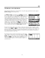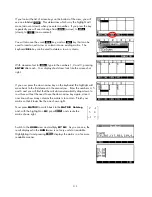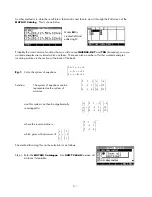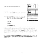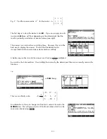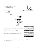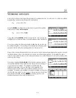
For example, suppose we use the system of equations below, in which the third equation is a linear
combination of the first two but the constant is not consistent with this - ie no solution.
⎧ + + =
5
If we solve this in the same way as before, the matrix
x
y
z
⎨
2
x
y
⎪
− = −
6
which results is:
⎪
+
⎩
3
2
13
y
z
=
The final line of [0 0 0 1] indicates no solution. See the chapter
“Working with Matrices” for more examples.
See also:
INVERSE
,
DET
SCHUR(<matrix>)
This function returns the Schur Decomposition for the square matrix supplied. The result is two matrices stored
in a list. If the supplied matrix is real, then the result is:
{[[orthogonal]],[[upper-quasi triangular]]}.
If matrix is complex, then the result is:
{[[unitary]],[[upper-triangular]]}.
SIZE(<list>) or SIZE(<matrix>)
This function returns the size of the list or matrix specified. Since normal
users would probably know anyway, and could find out easily via the list
catalog, this is clearly another of those functions which are of more use
to programmers (who won’t know when they write their program just
how long the list you will ask it to deal with will be when you eventually
run the program). If the object is a matrix then the return value is a two
element list as {rows, columns}.
SPECNORM(<matrix>)
This function returns the Spectral norm of a matrix.
SPECRAD(<matrix>)
This function returns the Spectral radius of a matrix.
200


