Page 6-29
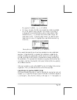
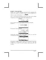
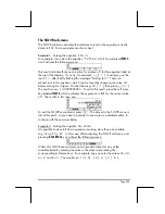
As variables Q, a, and b, get assigned numerical values, the assignments are
listed in the upper left corner of the display. At this point we can solve for t, by
using
„
[ t ]. The result is t: 2. Pressing
@EXPR=
shows the results:
Example 3 - Solving two simultaneous equations, one at a time
You can also solve more than one equation by solving one equation at a time,
and repeating the process until a solution is found. For example, if you enter
the following list of equations into variable EQ: { ‘a*X+b*Y = c’, ‘k*X*Y=s’},
the keystroke sequence
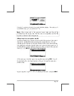
@)ROOT @)SOLVR
, within the SOLVE soft menu, will produce
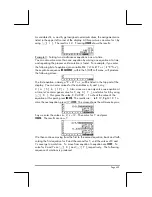
the following screen:
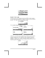
The first equation, namely, a*X + b*Y = c, will be listed in the top part of the
display. You can enter values for the variables a, b, and c, say:
2 [ a ] 5 [ b ] 19 [ c ]. Also, since we can only solve one equation at
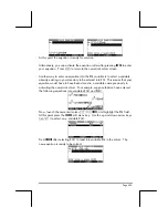
a time, let’s enter a guess value for Y, say, 0 [ Y ], and solve for X, by using
„
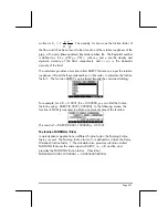
[ X ]. This gives the value, X: 9.4999…. To check the value of the
equation at this point, press
@EXPR=
. The results are: Left: 19, Right: 19. To
solve the next equation, press
L
@NEXQ
. The screen shows the soft menu keys as:
Say we enter the values k = 2, s = 12. Then solve for Y, and press
@EXPR=
. The results are now, Y:
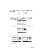
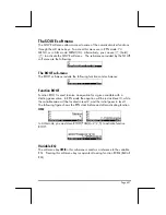
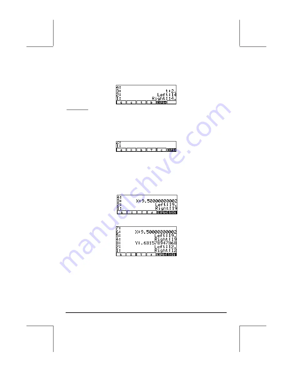
We then continue moving from the first to the second equation, back and forth,
solving the first equation for X and the second for Y, until the values of X and
Y converge to a solution. To move from equation to equation use
@NEXQ
. To
solve for X and Y use
„
[ X ], and
„
[ Y ], respectively. The following
sequence of solutions is produced:


