Page 18-55
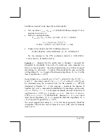
Confidence intervals for the slope (
Β
) and intercept (A):
•
First, we obtain t
n-2,
α
/2
= t
3
,
0.025
= 3.18244630528 (See chapter 17 for a
program to solve for t
ν
,a
):
•
Next, we calculate the terms
(t
n-2,
α
/2
)
⋅
s
e
/
√
S
xx
= 3.182…
⋅
(0.1826…/2.5)
1/2
= 0.8602…
(t
n-2,
α
/2
)
⋅
s
e
⋅
[(1/n)+
x
2
/S
xx
]
1/2
=
3.1824…
⋅√0
.1826…
⋅
[(1/5)+3
2
/2.5]
1/2
= 2.65
•
Finally, for the slope B, the 95% confidence interval is
(-0.86-0.860242, -0.86+0.860242) = (-1.72, -0.00024217)
For the intercept A, the 95% confidence interval is (3.24-2.6514,
3.24+2.6514) = (0.58855,5.8914).
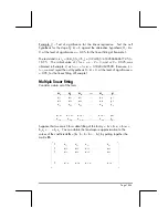
Example 2 -- Suppose that the y-data used in Example 1 represent the
elongation (in hundredths of an inch) of a metal wire when subjected to a
force x (in tens of pounds). The physical phenomenon is such that we expect
the intercept, A, to be zero. To check if that should be the case, we test the
null hypothesis, H
0
:
Α
=
0
, against the alternative hypothesis, H
1
:
Α
≠
0, at the
level of significance
α
= 0.05.
The test statistic is t
0
= (a-
0
)/[(1/n)+
x
2
/S
xx
]
1/2
= (-0.86)/ [(1/5)+3
2
/2.5]
½
= -
0.44117. The critical value of t, for
ν
= n – 2 = 3, and
α
/2 = 0.025, can
be calculated using the numerical solver for the equation
α
= UTPT(
γ
,t)
developed in Chapter 17. In this program,
γ
represents the degrees of
freedom (n-2), and
α
represents the probability of exceeding a certain value
of t, i.e., Pr[ t>t
α
] = 1 –
α
. For the present example, the value of the level of
significance is
α
= 0.05, g = 3, and t
n-2,
α
/2
= t
3,0.025
. Also, for
γ
= 3 and
α
=
0.025, t
n-2,
α
/2
= t
3,0.025
= 3.18244630528. Because t
0
> - t
n-2,
α
/2
, we cannot
reject the null hypothesis, H
0
:
Α
=
0
, against the alternative hypothesis, H
1
:
Α
≠
0, at the level of significance
α
= 0.05.
This result suggests that taking A = 0 for this linear regression should be
acceptable. After all, the value we found for a, was –0.86, which is relatively
close to zero.


